The era of large language models (LLMs) is here, bringing with it rapidly evolving libraries like ChromaDB that help augment LLM applications. You’ve most likely heard of chatbots like OpenAI’s ChatGPT, and perhaps you’ve even experienced their remarkable ability to reason about natural language processing (NLP) problems.
Modern LLMs, while imperfect, can accurately solve a wide range of problems and provide correct answers to many questions. But, due to the limits of their training and the number of text tokens they can process, LLMs aren’t a silver bullet for all tasks.
You wouldn’t expect an LLM to provide relevant responses about topics that don’t appear in their training data. For example, if you asked ChatGPT to summarize information in confidential company documents, then you’d be out of luck. You could show some of these documents to ChatGPT, but there’s a limited number of documents that you can upload before you exceed ChatGPT’s maximum number of tokens. How would you select documents to show ChatGPT?
To address these shortcomings and scale your LLM applications, one great option is to use a vector database like ChromaDB. A vector database allows you to store encoded unstructured objects, like text, as lists of numbers that you can compare to one another. You can, for example, find a collection of documents relevant to a question that you want an LLM to answer.
In this tutorial, you’ll learn about:
- Representing unstructured objects with vectors
- Using word and text embeddings in Python
- Harnessing the power of vector databases
- Encoding and querying over documents with ChromaDB
- Providing context to LLMs like ChatGPT with ChromaDB
After reading, you’ll have the foundational knowledge to use ChromaDB in your NLP or LLM applications. Before reading, you should be comfortable with the basics of Python and high school math.
Get Your Code: Click here to download free sample code that shows you how to use ChromaDB to add context to an LLM.
Represent Data as Vectors
Before diving into embeddings and vector databases, you should understand what vectors are and what they represent. Feel free to skip ahead to the next section if you’re already comfortable with vector concepts. If you’re not or if you could use a refresher, then keep reading!
Vector Basics
You can describe vectors with variable levels of complexity, but one great starting place is to think of a vector as an array of numbers. For example, you could represent vectors using NumPy arrays as follows:
>>> import numpy as np

>>> vector1 = np.array([1, 0])
>>> vector2 = np.array([0, 1])
>>> vector1
array([1, 0])

>>> vector2
array([0, 1])
In this code block, you import numpy and create two arrays, vector1 and vector2, representing vectors. This is one of the most common and useful ways to work with vectors in Python, and NumPy offers a variety of functionality to manipulate vectors. There are also several other libraries that you can use to work with vector data, such as PyTorch, TensorFlow, JAX, and Polars. You’ll stick with NumPy for this overview.
You’ve created two NumPy arrays that represent vectors. Now what? It turns out you can do a lot of cool things with vectors, but before continuing on, you’ll need to understand some key definitions and properties:
-
Dimension: The dimension of a vector is the number of elements that it contains. In the example above,
vector1andvector2are both two-dimensional since they each have two elements. You can only visualize vectors with three dimensions or less, but generally, vectors can have any number of dimensions. In fact, as you’ll see later, vectors that encode words and text tend to have hundreds or thousands of dimensions. -
Magnitude: The magnitude of a vector is a non-negative number that represents the vector’s size or length. You can also refer to the magnitude of a vector as the norm, and you can denote it with ||v|| or |v|. There are many different definitions of magnitude or norm, but the most common is the Euclidean norm or 2-norm. You’ll learn how to compute this later.
-
Unit vector: A unit vector is a vector with a magnitude of one. In the example above,
vector1andvector2are unit vectors. -
Direction: The direction of a vector specifies the line along which the vector points. You can represent direction using angles, unit vectors, or coordinates in different coordinate systems.
-
Dot product (scalar product): The dot product of two vectors, u and v, is a number given by u ⋅ v = ||u|| ||v|| cos(θ), where θ is the angle between the two vectors. Another way to compute the dot product is to do an element-wise multiplication of u and v and sum the results. The dot product is one of the most important and widely used vector operations because it measures the similarity between two vectors. You’ll see more of this later on.
-
Orthogonal vectors: Vectors are orthogonal if their dot product is zero, meaning that they’re at a 90 degree angle to each other. You can think of orthogonal vectors as being completely unrelated to each other.
-
Dense vector: A vector is considered dense if most of its elements are non-zero. Later on, you’ll see that words and text are most usefully represented with dense vectors because each dimension encodes meaningful information.
While there are many more definitions and properties to learn, these six are most important for this tutorial. To solidify these ideas with code, check out the following block. Note that for the rest of this tutorial, you’ll use v1, v2, and v3 to name your vectors:
>>> import numpy as np

>>> v1 = np.array([1, 0])
>>> v2 = np.array([0, 1])
>>> v3 = np.array([np.sqrt(2), np.sqrt(2)])

>>> # Dimension
>>> v1.shape
(2,)

>>> # Magnitude
>>> np.sqrt(np.sum(v1**2))
1.0
>>> np.linalg.norm(v1)
1.0

>>> np.linalg.norm(v3)
2.0

>>> # Dot product
>>> np.sum(v1 * v2)
0

>>> v1 @ v3
1.4142135623730951
You first import numpy and create the arrays v1, v2, and v3. Calling v1.shape shows you the dimension of v1. You then see two different ways to compute the magnitude of a NumPy array. The first, np.sqrt(np.sum(v1**2)), uses the Euclidean norm that you learned about above. The second computation uses np.linalg.norm(), a NumPy function that computes the Euclidean norm of an array by default but can also compute other matrix and vector norms.
Lastly, you see two ways to calculate the dot product between two vectors. Using np.sum(v1 * v2) first computes the element-wise multiplication between v1 and v2 in a vectorized fashion, and you sum the results to produce a single number. A better way to compute the dot product is to use the at-operator (@), as you see with v1 @ v3. This is because @ can perform both vector and matrix multiplications, and the syntax is cleaner.
While all of these vector definitions and properties may seem straightforward to compute, you might still be wondering what they actually mean and why they’re important to understand. One way to better understand vectors is to visualize them in two dimensions. In this context, you can represent vectors as arrows, like in the following plot:
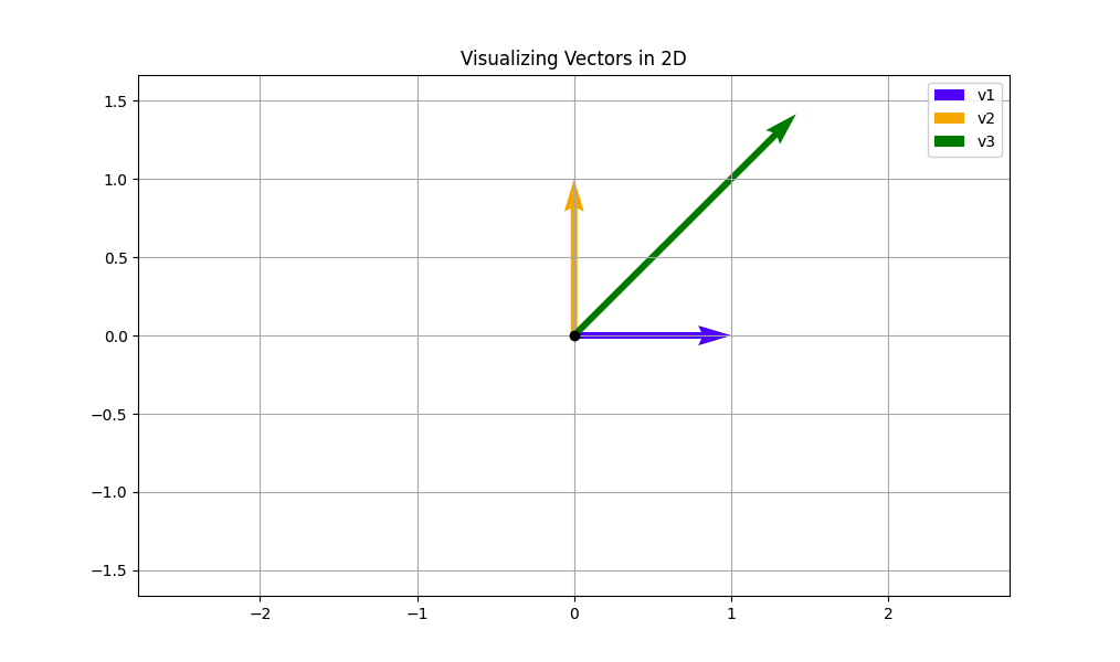
The above plot shows the visual representation of the vectors v1, v2, and v3 that you worked with in the last example. The tail of each vector arrow always starts at the origin, and the tip is located at the coordinates specified by the vector. As an example, the tip of v1 lies at (1, 0), and the tip of v3 lies at roughly (1.414, 1.414). The length of each vector arrow corresponds to the magnitude that you calculated earlier.
From this visual, you can make the following key inferences:
-
v1andv2are unit vectors because their magnitude, given by the arrow length, is one.v3isn’t a unit vector, and its magnitude is two, twice the size ofv1andv2. -
v1andv2are orthogonal because their tails meet at a 90 degree angle. You see this visually but can also verify it computationally by computing the dot product betweenv1andv2. By using the dot product definition, v1 ⋅ v2 = ||v1|| ||v2|| cos(θ), you can see that when θ = 90, cos(θ) = 0 and v1 ⋅ v2 = 0. Intuitively, you can think ofv1andv2as being totally unrelated or having nothing to do with each other. This will become important later. -
v3makes a 45 degree angle with bothv1andv2. This means thatv3will have a non-zero dot product withv1andv2. This also means thatv3is equally related to bothv1andv2. In general, the smaller the angle between two vectors, the more they point toward a common direction.
You’ve now seen how vectors are characterized both computationally and visually. With this understanding, you’re ready to take a slightly deeper dive into the idea of vector similarity. If you only take away one thing from this introduction, it should be what follows.
Vector Similarity
The ability to measure vector similarity is crucial in machine learning and mathematics more broadly. The foundation for this measurement lies in the dot product, which serves as the bedrock for many vector similarity metrics.
One issue with the dot product, when used in isolation, is that it can take on any value and is therefore difficult to interpret in absolute terms. For example, if you know only that the dot product between two vectors is -3, then it’s unclear what that means without more context.
To overcome this shortcoming, one common approach is to use cosine similarity, a normalized form of the dot product. You compute cosine similarity by taking the cosine of the angle between two vectors. In essence, you rearrange the cosine definition of the dot product from earlier to solve for cos(θ). The equation for cosine similarity looks like this:
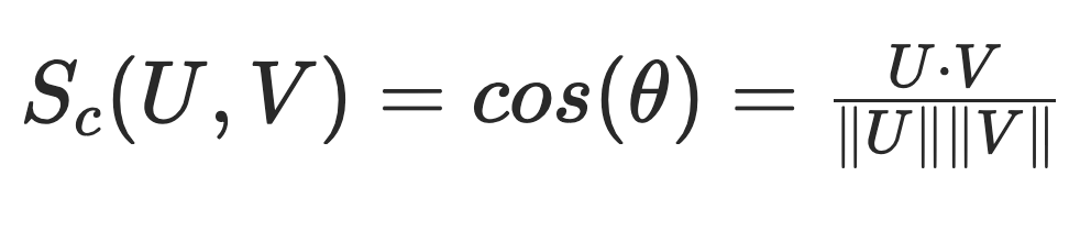
Cosine similarity disregards the magnitude of both vectors, forcing the calculation to lie between -1 and 1. This is a really nice property because it gives cosine similarity the following interpretations:
-
A value of 1 means the angle between the two vectors is 0 degrees. In other words, the two vectors are similar because they point in the exact same direction. Keep in mind this doesn’t mean that the vectors have the same magnitude.
-
A value of 0 means the angle between the two vectors is 90 degrees. In this case, the vectors are orthogonal and unrelated to each other.
-
A value of -1 means the angle between the two vectors is 180 degrees. This is an interesting case where the vectors are dissimilar because they point in opposite directions.
In short, a cosine similarity of 1 means the vectors are similar, 0 means the vectors are unrelated, and -1 means the vectors are opposite. Any values in between represent varying degrees of similarity or dissimilarity. Here’s a nice animation to solidify your idea of cosine similarity:
In this animation, vector U is fixed, while vector V rotates around it. At each rotation, the cosine similarity between U and V is calculated. As you can see, when U and V point in the same direction, the cosine similarity is 1. As V rotates past U in the counterclockwise direction, the cosine similarity decreases until it equals -1 when U and V point in opposite directions. When U and V are orthogonal, the cosine similarity is 0.
Note: The purpose of these examples is to deepen your understanding of vectors and vector similarity calculations. You used two-dimensional vectors because they’re straightforward to visualize, but keep in mind that everything covered so far applies to vectors of any dimension. In the next section, you’ll use the same cosine similarity calculation to compare vectors in high-dimensional vector spaces.
You now have a feel for what vectors are and how you can assess their similarity. While there are many more vector concepts to learn about, you know enough to speak the language of embeddings and vector databases. In the next section, you’ll see how to convert words and sentences to vectors, a key prerequisite to text-based vector databases.
Encode Objects in Embeddings
The next step in your journey to understanding and using vector databases like ChromaDB is to get a feel for embeddings. Embeddings are a way to represent data such as words, text, images, and audio in a numerical format that computational algorithms can more easily process.
More specifically, embeddings are dense vectors that characterize meaningful information about the objects that they encode. The most common kinds of embeddings are word and text embeddings, and that’s what you’ll focus on in this tutorial.
Word Embeddings
A word embedding is a vector that captures the semantic meaning of word. Ideally, words that are semantically similar in natural language should have embeddings that are similar to each other in the encoded vector space. Analogously, words that are unrelated or opposite of one another should be further apart in the vector space.
One of the best ways to conceptualize this idea is to plot example word vectors in two dimensions. Take a good look at this scatterplot:
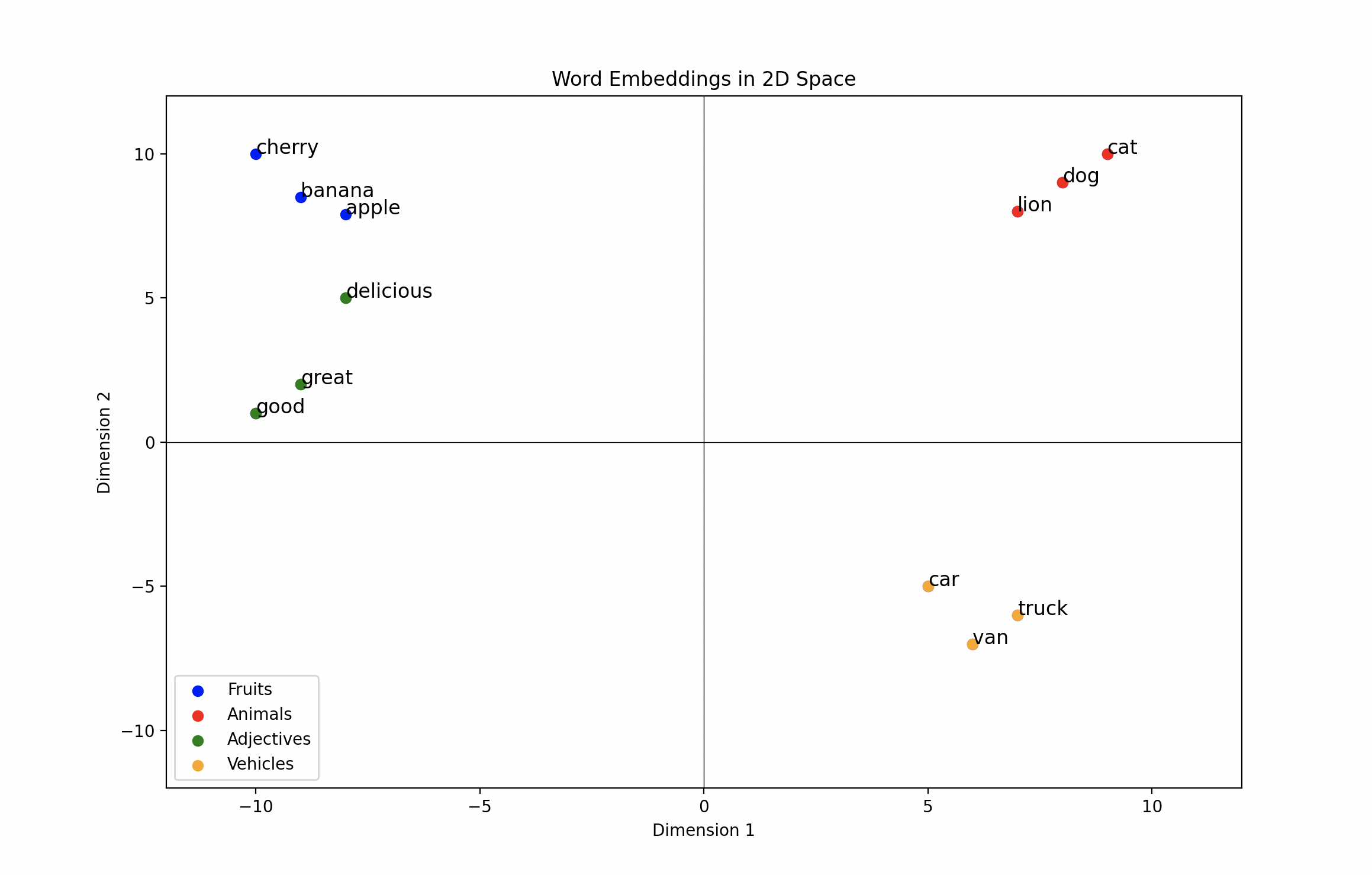
This plot shows hand-crafted word embeddings plotted in two dimensions. Each point indicates where the word embedding’s tail lies. You’ll notice how related words are clustered together, while unrelated words are far from each other.
As an example, the vehicle embeddings are far from the animal embeddings because there’s little semantic similarity between the two. On the other hand, the adjectives with positive connotations are relatively close to the fruits, with the delicious embedding being closest to the fruit embeddings.
Because you’ll usually find the word delicious in contexts relating to food, it makes sense for the delicious embedding to have some similarity with both food embeddings and positive adjective embeddings.
Word embeddings try to capture these semantic relationships for a large vocabulary of words, and as you might imagine, there are a lot of complex relationships to consider. This is why, in practice, word embeddings often require hundreds or thousands of dimensions to account for the complexities of human language.
Note: If you’re interested in how word embeddings are created, then check out the Word2vec and GloVe algorithms. These algorithms create static word embeddings like the ones that you’ll use later in this section, but there are other ways to create dynamic embeddings. For example, the model underlying most large language models (LLMs), including ChatGPT, creates word embeddings that change based on the context surrounding the word.
You’re now ready to get started using word vectors in Python. For this, you’ll use the popular spaCy library, a general-purpose NLP library. To install spaCy, create a virtual environment, activate it, and run the following command:
(venv) $ python -m pip install spacy
After you’ve installed spaCy, you’ll also need to download a model that provides word embeddings, among other features. For this tutorial, you’ll want to install the medium or large English model:
(venv) $ python -m spacy download en_core_web_md
SpaCy’s en_core_web_md model includes 20,000 pre-trained word embeddings, each of which has 300 dimensions. This is more than enough for the examples that you’ll see next, but if you have the appetite for more word embeddings, then you can download the en_core_web_lg model, which has 514,000 embeddings.
With spaCy’s medium or large English model installed, you’re ready to get started using word embeddings. It only takes a few lines of code to look up embeddings:
>>> import spacy

>>> nlp = spacy.load("en_core_web_md")

>>> dog_embedding = nlp.vocab["dog"].vector

>>> type(dog_embedding)
<class 'numpy.ndarray'>

>>> dog_embedding.shape
(300,)

>>> dog_embedding[0:10]
array([  1.233  ,   4.2963 ,  -7.9738 , -10.121  ,   1.8207 ,   1.4098 ,
        -4.518  ,  -5.2261 ,  -0.29157,   0.95234], dtype=float32)
You first import spacy and load the medium English model into an object called nlp. You then look up the embedding for the word dog with nlp.vocab["dog"].vector and store it as dog_embedding. Calling type(dog_embedding) tells you that the embedding is a NumPy array, and dog_embedding.shape indicates that the embedding has 300 dimensions. Lastly, dog_embedding[0:10] shows the values of the first 10 dimensions.
This is pretty neat! The nlp.vocab object allows you to find the word embedding for any word in the model’s vocabulary. You can now assess the similarity between word embeddings using metrics like cosine similarity. To do this, create a new file called cosine_similarity.py in your working directory that contains the following function:
cosine_similarity.py
import numpy as np

def compute_cosine_similarity(u: np.ndarray, v: np.ndarray) -> float:
    """Compute the cosine similarity between two vectors"""

    return (u @ v) / (np.linalg.norm(u) * np.linalg.norm(v))
This function computes the cosine similarity between two NumPy arrays, u and v, using the definition discussed previously. You can pass word embeddings directly from spaCy into compute_cosine_similarity() to see how related they are:
>>> import spacy
>>> from cosine_similarity import compute_cosine_similarity

>>> nlp = spacy.load("en_core_web_md")

>>> dog_embedding = nlp.vocab["dog"].vector
>>> cat_embedding = nlp.vocab["cat"].vector
>>> apple_embedding = nlp.vocab["apple"].vector
>>> tasty_embedding = nlp.vocab["tasty"].vector
>>> delicious_embedding = nlp.vocab["delicious"].vector
>>> truck_embedding = nlp.vocab["truck"].vector

>>> compute_cosine_similarity(dog_embedding, cat_embedding)
0.8220817

>>> compute_cosine_similarity(delicious_embedding, tasty_embedding)
0.8482092

>>> compute_cosine_similarity(apple_embedding, delicious_embedding)
0.5347655

>>> compute_cosine_similarity(dog_embedding, apple_embedding)
0.22881003

>>> compute_cosine_similarity(truck_embedding, delicious_embedding)
0.08978759
In this block, you import spacy and compute_cosine_similarity(), and you instantiate an nlp object using the medium-size English model. Next, you look up and store embeddings for six common words from the model’s vocabulary. By computing the cosine similarity between these embeddings, you get a sense for how the model views their semantic relationship. Here are some important observations about the similarity scores:
-
The cat and dog embeddings have a relatively high cosine similarity. This is likely because cats and dogs are common house pets, and you can find the word dog close to the word cat in English texts.
-
The delicious and tasty embeddings also have a high cosine similarity because they have almost the same meaning. However, unlike the dog and cat embeddings, delicious and tasty have similar word embeddings because you can use them interchangeably.
-
The delicious and apple embeddings have a moderate cosine similarity near 0.53. This is because delicious is a commonly used adjective to describe an apple. The reason that the cosine similarity isn’t higher in this case may be because apple and delicious aren’t always used in the same context. The word delicious can describe any food, not just apples.
-
The truck and delicious embeddings have a cosine similarity close to 0. As you might expect, truck and delicious aren’t words that commonly appear in the same context.
Word embeddings are great for capturing the semantic relationships between words, but what if you wanted to take things to the next level and analyze the similarity between sentences or documents? It turns out you accomplish this with text embeddings, and these are the kinds of embeddings that you’ll most often store in vector databases. More on that in the next section.
Text Embeddings
Text embeddings encode information about sentences and documents, not just individual words, into vectors. This allows you to compare larger bodies of text to each other just like you did with word vectors. Because they encode more information than a single word embedding, text embeddings are a more powerful representation of information.
Text embeddings are typically the fundamental objects stored in vector databases like ChromaDB, and in this section, you’ll learn how to create and compare them.
Note: If you’re curious about how the leap from word embeddings to text embeddings happens, then check out some of the publications on popular text embedding models. The best text embedding models are built using transformers, which leverage a mechanism known as attention. To oversimplify things, the attention mechanism helps create context-specific word embeddings that fuse into text embeddings.
The most efficient way to generate text embeddings is to use pretrained models. These models vary in size, but they’re all typically trained on a large corpus of text, enabling them to pick up on complex semantic relationships. The SentenceTransformers library in Python is one of the best tools for this. You can install sentence-transformers with the following command:
(venv) $ python -m pip install sentence-transformers
Generating text embeddings with SentenceTransformers is just as straightforward as using word vectors in spaCy. Here’s an example to get you started:
>>> from sentence_transformers import SentenceTransformer

>>> model = SentenceTransformer("all-MiniLM-L6-v2")
>>> texts = [
...          "The canine barked loudly.",
...          "The dog made a noisy bark.",
...          "He ate a lot of pizza.",
...          "He devoured a large quantity of pizza pie.",
... ]

>>> text_embeddings = model.encode(texts)

>>> type(text_embeddings)
<class 'numpy.ndarray'>

>>> text_embeddings.shape
(4, 384)
You first import the SentenceTransformer class and load the "all-MiniLM-L6-v2" model into an object called model. This is one of the smallest pretrained models available, but it’s a great one to start with.
Note: The first time you use a model in SentenceTransformers, you’ll automatically download and save it in your environment. The initial download will take a few seconds depending on how large the model is, but after that, the model should load quickly.
Next, you define a list of sentences and call model.encode(texts) to create the corresponding text embeddings. Notice that text_embeddings is a NumPy array with the shape (4, 384), which means that it has 4 rows and 384 columns. This is because you encoded 4 texts, and "all-MiniLM-L6-v2" generates 384-dimensional embeddings.
While all the texts in this example are single sentences, you can encode longer texts up to a specified word length. For example, "all-MiniLM-L6-v2" encodes texts up to 256 words. It’ll truncate any text longer than this.
You now have a text embedding for all four texts, and just like with word embeddings, you can compare them using cosine similarity:
>>> from cosine_similarity import compute_cosine_similarity

>>> text_embeddings_dict = dict(zip(texts, list(text_embeddings)))

>>> dog_text_1 = "The canine barked loudly."
>>> dog_text_2 = "The dog made a noisy bark."
>>> compute_cosine_similarity(text_embeddings_dict[dog_text_1],
...                           text_embeddings_dict[dog_text_2])
0.77686167

>>> pizza_text_1 = "He ate a lot of pizza."
>>> pizza_test_2 = "He devoured a large quantity of pizza pie."
>>> compute_cosine_similarity(text_embeddings_dict[pizza_text_1],
...                           text_embeddings_dict[pizza_test_2])
0.78713405

>>> compute_cosine_similarity(text_embeddings_dict[dog_text_1],
...                           text_embeddings_dict[pizza_text_1])
0.0912827
After importing compute_cosine_similarity(), you use dict() and zip() together to create a dictionary where the keys are the four sentences and the values are their embeddings. This allows you to directly look up the embeddings for each text. You then compute the cosine similarity between a few pairs of texts. Here are some important conclusions:
-
The cosine similarity between The canine barked loudly and The dog made a noisy bark is relatively high even though the two sentences use different words. The same is true for the similarity between He ate a lot of pizza and He devoured a large quantity of pizza pie. Because the text embeddings encode semantic meaning, any pair of related texts should have a high cosine similarity.
-
As you might expect, the cosine similarity between The canine barked loudly and He ate a lot of pizza is low because the sentences are unrelated to each other.
This example, while straightforward, illustrates a powerful idea that underpins vector databases. That is, you can take a collection of unstructured objects, compute and store their embeddings, and then compare these embeddings to one another or to new embeddings. In this case, the unstructured objects are text, but keep in mind that the same idea can work for other data like images and audio.
Now that you’re up to speed on vectors and embeddings, you’re ready to get started with ChromaDB! In the next section, you’ll learn about vector databases and get a hands-on overview of ChromaDB.
Get Started With ChromaDB, an Open-Source Vector Database
Now that you understand the mechanisms behind ChromaDB, you’re ready to tackle a real-world scenario. Say you have a library of thousands of documents, and you need a way to search through them.
In particular, you want to be able to make queries that point you to relevant documents. For example, if your query is find me documents containing financial information, then you want whatever system you use to point you to a financial document in your library.
How would you design this system? With your knowledge of vectors and embeddings, your first inclination might be to run all of the documents through an embedding algorithm and store the documents and embeddings together. You’d then convert a new query to an embedding and use cosine similarity to find the documents that are most relevant to the query.
While you’re perfectly capable of writing the code for this, you’re sure there has to be something out there to do this for you. Enter vector databases!
What Is a Vector Database?
A vector database is a database that allows you to efficiently store and query embedding data. Vector databases extend the capabilities of traditional relational databases to embeddings. However, the key distinguishing feature of a vector database is that query results aren’t an exact match to the query. Instead, using a specified similarity metric, the vector database returns embeddings that are similar to a query.
As an example use case, suppose you’ve stored company documents in a vector database. This means each document has been embedded and can be compared to other embeddings through a similarity metric like cosine similarity.
The vector database will accept a query like how much revenue did the company make in Q2 2023 and embed the query. It’ll then compare the embedded query to other embeddings in the vector database and return the documents that have embeddings that are most similar to the query embedding.
In this example, perhaps the most similar document says something like Company XYZ reported $15 million in revenue for Q2 2023. The vector database identified the document that had an embedding most similar to how much revenue did the company make in Q2 2023, which likely had a high similarity score based on the document’s semantics.
To make this possible, vector databases are equipped with features that balance the speed and accuracy of query results. Here are the core components of a vector database that you should know about:
-
Embedding function: When using a vector database, oftentimes you’ll store and query data in its raw form, rather than uploading embeddings themselves. Internally, the vector database needs to know how to convert your data to embeddings, and you have to specify an embedding function for this. For text, you can use the embedding functions available in the SentenceTransformers library or any other function that maps raw text to vectors.
-
Similarity metric: To assess embedding similarity, you need a similarity metric like cosine similarity, the dot product, or Euclidean distance. As you learned previously, cosine similarity is a popular choice, but choosing the right similarity metric depends on your application.
-
Indexing: When you’re dealing with a large number of embeddings, comparing a query embedding to every embedding stored in the database is often too slow. To overcome this, vector databases employ indexing algorithms that group similar embeddings together.
At query time, the query embedding is compared to a smaller subset of embeddings based on the index. Because the embeddings recommended by the index aren’t guaranteed to have the highest similarity to the query, this is called approximate nearest neighbor search.
-
Metadata: You can store metadata with each embedding to help give context and make query results more precise. You can filter your embedding searches on metadata much like you would in a relational database. For example, you could store the year that a document was published as metadata and only look for similar documents that were published in a given year.
-
Storage location: With any kind of database, you need a place to store the data. Vector databases can store embeddings and metadata both in memory and on disk. Keeping data in memory allows for faster reads and writes, while writing to disk is important for persistent storage.
-
CRUD operations: Most vector databases support create, read, update, and delete (CRUD) operations. This means you can maintain and interact with data like you would in a relational database.
There’s a whole lot more detail and complexity that you could explore with vector databases, but these core concepts should be enough to get you going. Next up, you’ll get your hands dirty with ChromaDB, one of the most popular and user-friendly vector databases around.
Meet ChromaDB for LLM Applications
ChromaDB is an open-source vector database designed specifically for LLM applications. ChromaDB offers you both a user-friendly API and impressive performance, making it a great choice for many embedding applications. To get started, activate your virtual environment and run the following command:
(venv) $ python -m pip install chromadb
If you have any issues installing ChromaDB, take a look at the troubleshooting guide for help.
Because you have a grasp on vectors and embeddings, and you understand the motivation behind vector databases, the best way to get started is with an example. For this example, you’ll store ten documents to search over. To illustrate the power of embeddings and semantic search, each document covers a different topic, and you’ll see how well ChromaDB associates your queries with similar documents.
You’ll start by importing dependencies, defining configuration variables, and creating a ChromaDB client:
>>> import chromadb
>>> from chromadb.utils import embedding_functions

>>> CHROMA_DATA_PATH = "chroma_data/"
>>> EMBED_MODEL = "all-MiniLM-L6-v2"
>>> COLLECTION_NAME = "demo_docs"

>>> client = chromadb.PersistentClient(path=CHROMA_DATA_PATH)
You first import chromadb and then import the embedding_functions module, which you’ll use to specify the embedding function. Next, you specify the location where ChromaDB will store the embeddings on your machine in CHROMA_DATA_PATH, the name of the embedding model that you’ll use in EMBED_MODEL, and the name of your first collection in COLLECTION_NAME.
You then instantiate a PersistentClient object that writes your embedding data to CHROMA_DB_PATH. By doing this, you ensure that data will be stored at CHROMA_DB_PATH and persist to new clients. Alternatively, you can use chromadb.Client() to instantiate a ChromaDB instance that only writes to memory and doesn’t persist on disk.
Next, you instantiate your embedding function and the ChromaDB collection to store your documents in:
>>> embedding_func = embedding_functions.SentenceTransformerEmbeddingFunction(
...     model_name=EMBED_MODEL
... )

>>> collection = client.create_collection(
...     name=COLLECTION_NAME,
...     embedding_function=embedding_func,
...     metadata={"hnsw:space": "cosine"},
... )
You specify an embedding function from the SentenceTransformers library. ChromaDB will use this to embed all your documents and queries. In this example, you’ll continue using the "all-MiniLM-L6-v2" model. You then create your first collection.
A collection is the object that stores your embedded documents along with any associated metadata. If you’re familiar with relational databases, then you can think of a collection as a table. In this example, your collection is named demo_docs, it uses the "all-MiniLM-L6-v2" embedding function that you instantiated, and it uses the cosine similarity distance function as specified by metadata={"hnsw:space": "cosine"}.
The last step in setting up your collection is to add documents and metadata:
>>> documents = [
...     "The latest iPhone model comes with impressive features and a powerful camera.",
...     "Exploring the beautiful beaches and vibrant culture of Bali is a dream for many travelers.",
...     "Einstein's theory of relativity revolutionized our understanding of space and time.",
...     "Traditional Italian pizza is famous for its thin crust, fresh ingredients, and wood-fired ovens.",
...     "The American Revolution had a profound impact on the birth of the United States as a nation.",
...     "Regular exercise and a balanced diet are essential for maintaining good physical health.",
...     "Leonardo da Vinci's Mona Lisa is considered one of the most iconic paintings in art history.",
...     "Climate change poses a significant threat to the planet's ecosystems and biodiversity.",
...     "Startup companies often face challenges in securing funding and scaling their operations.",
...     "Beethoven's Symphony No. 9 is celebrated for its powerful choral finale, 'Ode to Joy.'",
... ]

>>> genres = [
...     "technology",
...     "travel",
...     "science",
...     "food",
...     "history",
...     "fitness",
...     "art",
...     "climate change",
...     "business",
...     "music",
... ]

>>> collection.add(
...     documents=documents,
...     ids=[f"id{i}" for i in range(len(documents))],
...     metadatas=[{"genre": g} for g in genres]
... )
In this block, you define a list of ten documents in documents and specify the genre of each document in genres. You then add the documents and genres using collection.add(). Each document in the documents argument is embedded and stored in the collection. You also have to define the ids argument to uniquely identify each document and embedding in the collection. You accomplish this with a list comprehension that creates a list of ID strings.
The metadatas argument is optional, but most of the time, it’s useful to store metadata with your embeddings. In this case, you define a single metadata field, "genre", that records the genre of each document. When you query a document, metadata provides you with additional information that can be helpful to better understand the document’s contents. You can also filter on metadata fields, just like you would in a relational database query.
With documents embedded and stored in a collection, you’re ready to run some semantic queries:
>>> query_results = collection.query(
...     query_texts=["Find me some delicious food!"],
...     n_results=1,
... )

>>> query_results.keys()
dict_keys(['ids', 'distances', 'metadatas', 'embeddings', 'documents'])

>>> query_results["documents"]
[['Traditional Italian pizza is famous for its thin crust, fresh ingredients, and wood-fired ovens.']]

>>> query_results["ids"]
[['id3']]

>>> query_results["distances"]
[[0.7638263782124082]]

>>> query_results["metadatas"]
[[{'genre': 'food'}]]
In this example, you query the demo_docs collection for documents that are most similar to the sentence Find me some delicious food!. You accomplish this using collection.query(), where you pass your queries in query_texts and specify the number of similar documents to find with n_results. In this case, you only asked for the single document that’s most similar to your query.
The results returned by collection.query() are stored in a dictionary with the keys ids, distances, metadatas, embeddings, and documents. This is the same information that you added to your collection at the beginning, but it’s filtered down to match your query. In other words, collection.query() returns all of the stored information about documents that are most similar to your query.
As you can see, the embedding for Traditional Italian pizza is famous for its thin crust, fresh ingredients, and wood-fired ovens was most similar to the query Find me some delicious food. You probably agree that this document is the closest match. You can also see the ID, metadata, and distance associated with the matching document embedding. Here, you’re using cosine distance, which is one minus the cosine similarity between two embeddings.
With collection.query(), you’re not limited to single queries or single results:
>>> query_results = collection.query(
...     query_texts=["Teach me about history",
...                  "What's going on in the world?"],
...     include=["documents", "distances"],
...     n_results=2
... )

>>> query_results["documents"][0]
[
  "Einstein's theory of relativity revolutionized our understanding of space and time.",
  "The American Revolution had a profound impact on the birth of the United States as a nation."
]

>>> query_results["distances"][0]
[0.6265882306931405, 0.6904192942966181]

>>> query_results["documents"][1]
[
  "Climate change poses a significant threat to the planet's ecosystems and biodiversity.",
  "Einstein's theory of relativity revolutionized our understanding of space and time."
]

>>> query_results["distances"][1]
[0.8002944367743202, 0.8882106528891986]
Here, you pass two queries into collection.query(), Teach me about history and What’s going on in the world. You also request the two most similar documents for each query by specifying n_results=2. Lastly, by passing include=["documents", "distances"], you ensure that the dictionary only contains the documents and their embedding distances.
Calling query_results["documents"][0] shows you the two most similar documents to the first query in query_texts, and query_results["distances"][0] contains the corresponding embedding distances. As an example, the cosine distance between Teach me about history and Einstein’s theory of relativity revolutionized our understanding of space and time is about 0.627.
Similarly, query_results["documents"][1] shows you the two most similar documents to the second query in query_texts, and query_results["distances"][1] contains the corresponding embedding distances. For this query, the two most similar documents weren’t as strong of a match as in the first query. Recall that cosine distance is one minus cosine similarity, so a cosine distance of 0.80 corresponds to a cosine similarity of 0.20.
Note: Keep in mind that so-called similar documents returned from a semantic search over embeddings may not actually be relevant to the task that you’re trying to solve. The success of a semantic search is somewhat subjective, and you or your stakeholders might not agree on the quality of the results.
If there are no relevant documents in your collection for a given query, or your embedding algorithm wasn’t trained on the right or enough data, then your results might be poor. It’s up to you to understand your application, your stakeholders’ expectations, and the limitations of your embedding algorithm and document collection.
Another awesome feature of ChromaDB is the ability to filter queries on metadata. To motivate this, suppose you want to find the single document that’s most related to music history. You might run this query:
>>> collection.query(
...     query_texts=["Teach me about music history"],
...     n_results=1
... )
{
 'ids': [['id2']],
 'distances': [[0.7625819917739272]],
 'metadatas': [[{'genre': 'science'}]],
 'embeddings': None,
 'documents': [["Einstein's theory of relativity revolutionized our understanding of space and time."]]
}
Your query is Teach me about music history, and the most similar document is Einstein’s theory of relativity revolutionized our understanding of space and time. While Einstein is a historical figure who was a musician and teacher, this isn’t quite the result that you’re looking for. Because you’re particularly interested in music history, you can filter on the "genre" metadata field to search over more relevant documents:
>>> collection.query(
...     query_texts=["Teach me about music history"],
...     where={"genre": {"$eq": "music"}},
...     n_results=1,
... )
{
 'ids': [['id9']],
 'distances': [[0.8186328925270356]],
 'metadatas': [[{'genre': 'music'}]],
 'embeddings': None,
 'documents': [["Beethoven's Symphony No. 9 is celebrated for its powerful choral finale, 'Ode to Joy.'"]]
}
In this query, you specify in the where argument that you’re only looking for documents with the "music" genre. To apply filters, ChromaDB expects a dictionary where the keys are metadata names and the values are dictionaries specifying how to filter. In plain English, you can interpret {"genre": {"$eq": "music"}} as filter the collection where the "genre" metadata field equals "music".
As you can see, the document about Beethoven’s Symphony No. 9 is the most similar document. Of course, for this example, there’s only one document with the music genre. To make it slightly more difficult, you could filter on both history and music:
>>> query_results = collection.query(
...     query_texts=["Teach me about music history"],
...     where={"genre": {"$in": ["music", "history"]}},
...     n_results=2,
... )

>>> query_results["documents"]
[
  [
    "Beethoven's Symphony No. 9 is celebrated for its powerful choral finale, 'Ode to Joy.'",
    'The American Revolution had a profound impact on the birth of the United States as a nation.'
  ]
]

>>> query_results["distances"]
[[0.8186329003249154, 0.8200413574222101]]
This query filters the collection of documents that have either a music or history genre, as specified by where={"genre": {"$in": ["music", "history"]}}. As you can see, the Beethoven document is still the most similar, while the American Revolution document is a close second. These were straightforward filtering examples on a single metadata field, but ChromaDB also supports other filtering operations that you might need.
If you want to update existing documents, embeddings, or metadata, then you can use collection.update(). This requires you to know the IDs of the data that you want to update. In this example, you’ll update both the documents and metadata for "id1" and "id2":
>>> collection.update(
...     ids=["id1", "id2"],
...     documents=["The new iPhone is awesome!",
...                "Bali has beautiful beaches"],
...     metadatas=[{"genre": "tech"}, {"genre": "beaches"}]
... )

>>> query_results = collection.get(ids=["id1", "id2"])

>>> query_results["documents"]
['The new iPhone is awesome!', 'Bali has beautiful beaches']

>>> query_results["metadatas"]
[{'genre': 'tech'}, {'genre': 'beaches'}]
Here, you rename the documents for "id1" and "id2", and you also modify their metadata. To confirm that your update worked, you call collection.get(ids=["id1", "id2"]) and can see that you’ve successfully updated both documents and their metadata. If you’re not sure whether a document exists for an ID, you can use collection.upsert(). This works the same way as collection.update(), except it’ll insert new documents for IDs that don’t exist.
Lastly, if you want to delete any items in the collection, then you can use collection.delete():
>>> collection.delete(ids=["id1", "id2"])

>>> collection.count()
8

>>> collection.get(["id1", "id2"])
{'ids': [], 'embeddings': None, 'metadatas': [], 'documents': []}
In this block, you use collection.delete(ids=["id1", "id2"]) to delete all data associated with "id1" and "id2". You then verify the deletion of these two documents by calling collection.count(), and you can see that collection.get(["id1", "id2"]) has no data.
You’ve now seen many of ChromaDB’s main features, and you can learn more with the getting started guide or API cheat sheet. You used a collection of ten hand-crafted documents that allowed you to get familiar with ChromaDB’s syntax and querying functionality, but this was by no means a realistic use case. In the next section, you’ll see ChromaDB shine while you embed and query over thousands of real-world documents!
Practical Example: Add Context for a Large Language Model (LLM)
Vector databases are capable of storing all types of embeddings, such as text, audio, and images. However, as you’ve learned, ChromaDB was initially designed with text embeddings in mind, and it’s most often used to build LLM applications. In this section, you’ll get hands-on experience using ChromaDB to provide context to OpenAI’s ChatGPT LLM.
To set the scene, you’re a data scientist who works for a large car dealership. The dealership has sold hundreds of thousands of cars and received many reviews. Your stakeholders would like you to create a system that summarizes different types of car reviews. They’ll use these summaries to improve marketing and prevent poor customer experiences in the future.
You’re responsible for designing and implementing the back-end logic that creates these summaries. You’ll take the following steps:
- Create a ChromaDB collection that stores car reviews along with associated metadata.
- Create a system that accepts a query, finds semantically similar documents, and uses the similar documents as context to an LLM. The LLM will use the documents to answer the question posed in the query.
This process of retrieving relevant documents and using them as context for a generative model is known as retrieval-augmented generation (RAG). This allows LLMs to make inferences using information that wasn’t included in their training dataset, and this is the most common way to apply ChromaDB in LLM applications.
There are lots of factors and variations to consider when implementing a RAG system, but for this example, you’ll only need to know the fundamentals. Here’s what a RAG system might look like with ChromaDB:
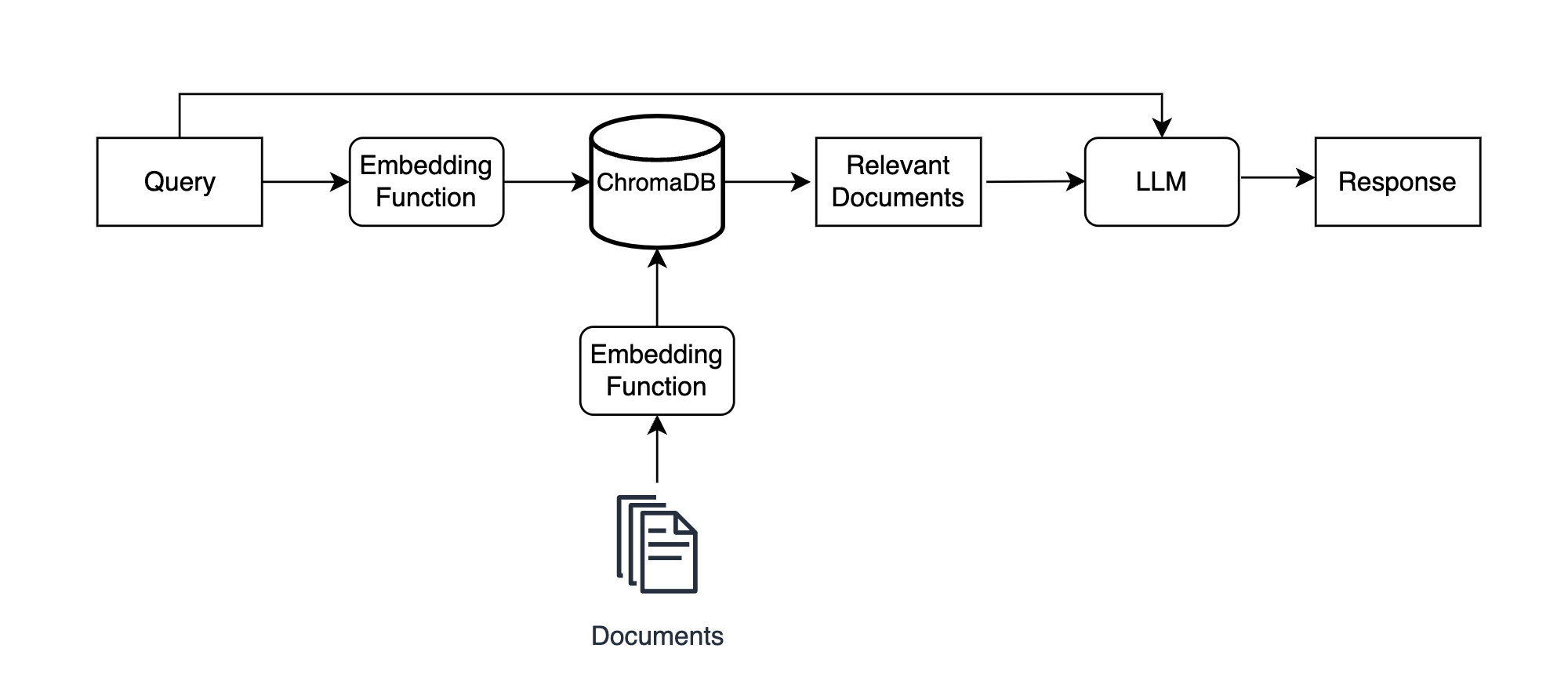
You first embed and store your documents in a ChromaDB collection. In this example, those documents are car reviews. You then run a query like find and summarize the best car reviews through ChromaDB to find semantically relevant documents, and you pass the query and relevant documents to an LLM to generate a context-informed response.
The key here is that the LLM takes both the original query and the relevant documents as input, allowing it to generate a meaningful response that it wouldn’t be able to create without the documents.
In reality, your deliverable for this project would likely be a chatbot that stakeholders use to ask questions about car reviews through a user interface. While building a full-fledged chatbot is beyond the scope of this tutorial, you can check out libraries like LangChain that are designed specifically to help you assemble LLM applications.
The focus of this example is for you to see how you can use ChromaDB for RAG. This practical knowledge will help reduce the learning curve for LangChain if you choose to go that route in the future. With that, you’re ready to get started!
Prepare and Inspect Your Dataset
You’ll use the Edmunds-Consumer Car Ratings and Reviews dataset from Kaggle to create the review collection. This dataset contains over 200,000 reviews and ratings covering 62 major car brands.
Once you’ve downloaded the dataset, unzip the file and store the data in your project directory inside a subdirectory called data/. There’s one CSV file per car, and you should store all of them within data/archive/.
To start, you can take a look at the dataset using Polars, a popular DataFrame library. Make sure that you have Polars installed in your environment:
(venv) $ python -m pip install polars
The focus of this tutorial isn’t on Polars, so you won’t get a detailed explanation of the Polars code. If you’re interested in learning more about Polars, then check out this Polars tutorial.
Here’s a function that you can use to prepare the car reviews dataset for ChromaDB:
car_data_etl.py
import pathlib
import polars as pl

def prepare_car_reviews_data(data_path: pathlib.Path, vehicle_years: list[int] = [2017]):
    """Prepare the car reviews dataset for ChromaDB"""

    # Define the schema to ensure proper data types are enforced
    dtypes = {
        "": pl.Int64,
        "Review_Date": pl.Utf8,
        "Author_Name": pl.Utf8,
        "Vehicle_Title": pl.Utf8,
        "Review_Title": pl.Utf8,
        "Review": pl.Utf8,
        "Rating": pl.Float64,
    }

    # Scan the car reviews dataset(s)
    car_reviews = pl.scan_csv(data_path, dtypes=dtypes)

    # Extract the vehicle title and year as new columns
    # Filter on selected years
    car_review_db_data = (
        car_reviews.with_columns(
            [
                (
                    pl.col("Vehicle_Title").str.split(
                        by=" ").list.get(0).cast(pl.Int64)
                ).alias("Vehicle_Year"),
                (pl.col("Vehicle_Title").str.split(by=" ").list.get(1)).alias(
                    "Vehicle_Model"
                ),
            ]
        )
        .filter(pl.col("Vehicle_Year").is_in(vehicle_years))
        .select(["Review_Title", "Review", "Rating", "Vehicle_Year", "Vehicle_Model"])
        .sort(["Vehicle_Model", "Rating"])
        .collect()
    )

    # Create ids, documents, and metadatas data in the format chromadb expects
    ids = [f"review{i}" for i in range(car_review_db_data.shape[0])]
    documents = car_review_db_data["Review"].to_list()
    metadatas = car_review_db_data.drop("Review").to_dicts()

    return {"ids": ids, "documents": documents, "metadatas": metadatas}
In your car_data_etl.py script, prepare_car_reviews_data() accepts the path to the car reviews dataset and a list of vehicle years to filter on, and it returns a dictionary with the review data properly formatted for ChromaDB. You can include different vehicle years, but keep in mind that the more years you include, the longer it’ll take to build the collection. By default, you’re only including vehicles from 2017.
You can see this function in action with the following code:
>>> from car_data_etl import prepare_car_reviews_data
>>> DATA_PATH = "data/archive/*"

>>> chroma_car_reviews_dict = prepare_car_reviews_data(DATA_PATH)
>>> chroma_car_reviews_dict.keys()
dict_keys(['ids', 'documents', 'metadatas'])

>>> chroma_car_reviews_dict["ids"][-10]
'review5860'

>>> print(chroma_car_reviews_dict["documents"][-10])
I've never had a perfect car for me but this is quite close. My husband
refused to ever drive an SUV but he loves this car. He's always looking
for an excuse to drive. It has power! There are lots of extras in the
inscription that are worth the extra money. I like the larger tires and
leather quality especially. My kids love the car too and prefer to ride
in the "way back". Some of the technology is tricky but you do get the
hang of it and there are so many features that it's worth the effort to
learn it.

>>> chroma_car_reviews_dict["metadatas"][-10]
{'Review_Title': 'Very happy!', 'Rating': 5.0, 'Vehicle_Year': 2017, 'Vehicle_Model': 'Volvo'}
In this block, you import prepare_car_reviews_data() from car_data_etl.py, store the path to the raw review CSV datasets, and create chroma_car_reviews_dict, which stores the reviews in a ChromaDB-compatible format. You then display the ID, document text, and metadata associated with one of the reviews.
Create a Collection and Add Reviews
Next, you’ll create a collection and add the reviews. This function will help you create a collection in a modular way. Before running this function, make sure you’ve installed more-itertools:
(venv) $ python -m pip install more-itertools
If you’re using Python 3.12 or higher, then you can use itertools.batched() to accomplish the same task as below. However, using more-itertools means that your code is fully backward compatible:
chroma_utils.py
 1import pathlib
 2import chromadb
 3from chromadb.utils import embedding_functions
 4from more_itertools import batched
 5
 6def build_chroma_collection(
 7    chroma_path: pathlib.Path,
 8    collection_name: str,
 9    embedding_func_name: str,
10    ids: list[str],
11    documents: list[str],
12    metadatas: list[dict],
13    distance_func_name: str = "cosine",
14):
15    """Create a ChromaDB collection"""
16
17    chroma_client = chromadb.PersistentClient(chroma_path)
18
19    embedding_func = embedding_functions.SentenceTransformerEmbeddingFunction(
20        model_name=embedding_func_name
21    )
22
23    collection = chroma_client.create_collection(
24        name=collection_name,
25        embedding_function=embedding_func,
26        metadata={"hnsw:space": distance_func_name},
27    )
28
29    document_indices = list(range(len(documents)))
30
31    for batch in batched(document_indices, 166):
32        start_idx = batch[0]
33        end_idx = batch[-1]
34
35        collection.add(
36            ids=ids[start_idx:end_idx],
37            documents=documents[start_idx:end_idx],
38            metadatas=metadatas[start_idx:end_idx],
39        )
In lines 1 to 4, you import the dependencies needed to define build_chroma_collection(). This function accepts the path where you’ll store the embeddings, the name of the collection to create, the name of the embedding function to use, the data to store in the collection, and the name of the distance function to use.
You then instantiate a PersistentClient() object, create the collection, and add data to the collection. In lines 29 to 39, you add data to the collection in batches using the more-itertools library. Calling batched(document_indices, 166) breaks document_indices into a list of tuples, each with size 166. ChromaDB’s current maximum batch size is 166, but this might change in the future.
You can now create the collection that stores car reviews:
>>> import chromadb
>>> from chromadb.utils import embedding_functions
>>> from car_data_etl import prepare_car_reviews_data
>>> from chroma_utils import build_chroma_collection

>>> DATA_PATH = "data/archive/*"
>>> CHROMA_PATH = "car_review_embeddings"
>>> EMBEDDING_FUNC_NAME = "multi-qa-MiniLM-L6-cos-v1"
>>> COLLECTION_NAME = "car_reviews"

>>> chroma_car_reviews_dict = prepare_car_reviews_data(DATA_PATH)

>>> build_chroma_collection(
...     CHROMA_PATH,
...     COLLECTION_NAME,
...     EMBEDDING_FUNC_NAME,
...     chroma_car_reviews_dict["ids"],
...     chroma_car_reviews_dict["documents"],
...     chroma_car_reviews_dict["metadatas"]
... )
As before, you import dependencies, define some configuration variables, and transform the raw reviews data. You then build a collection called car_review_embeddings using build_chroma_collection(). Notice that you’re now using the "multi-qa-MiniLM-L6-cos-v1" embedding function. The model behind this embedding function was specifically trained to solve question-and-answer semantic search tasks.
Building the collection will take a few minutes, but once it completes, you can run queries like the following:
>>> client = chromadb.PersistentClient(CHROMA_PATH)
>>> embedding_func = embedding_functions.SentenceTransformerEmbeddingFunction(
...         model_name=EMBEDDING_FUNC_NAME
...     )
>>> collection = client.get_collection(name=COLLECTION_NAME, embedding_function=embedding_func)

>>> great_reviews = collection.query(
...     query_texts=["Find me some positive reviews that discuss the car's performance"],
...     n_results=5,
...     include=["documents", "distances", "metadatas"]
... )

>>> great_reviews["documents"][0][0]
' Great all around car with great balance of performance and comfort. Terrific technology too.'
You query the car_reviews collection with Find me some positive reviews that discuss the car’s performance, and you display the most similar result. All of your reviews are now embedded, and you’re ready to integrate them into the summarization application.
Connect to an LLM Service
As you know, you’re going to use the car reviews as context to an LLM. This means that you’ll ask the LLM a question like How would you summarize the most common complaints from negative car reviews?, and you’ll provide relevant reviews to help the LLM answer this question. To do this, you’ll first need to install the openai library:
(venv) $ python -m pip install openai
You need an API key to interact with the models in the openai library, and you can check out this tutorial to help you get set up. Once you have your API key, you can store it as an environment variable or add it to a configuration file like this JSON file that you could name config.json:
config.json
{
    "openai-secret-key": "<your-api-key>"
}
To make sure your API works and everything is running properly, you can run the following code, which will ask the LLM a question without considering any of the documents in your ChromaDB collection:
>>> import os
>>> import json
>>> import openai
>>> os.environ["TOKENIZERS_PARALLELISM"] = "false"

>>> with open("config.json", mode="r") as json_file:
...     config_data = json.load(json_file)
...
>>> openai.api_key = config_data.get("openai-secret-key")
>>> context = "You are a customer success employee at a large car dealership."
>>> question = "What's the key to great customer satisfaction?"

>>> chat_response = openai.ChatCompletion.create(
...     model="gpt-3.5-turbo",
...     messages=[
...         {"role": "system", "content": context},
...         {"role": "user", "content": question},
...     ],
...     temperature=0,
...     n=1,
... )

>>> print(chat_response["choices"][0]["message"]["content"])
The key to great customer satisfaction is providing exceptional customer
service. This involves understanding and anticipating the needs of customers,
being responsive and attentive to their inquiries and concerns, and going
above and beyond to exceed their expectations. Building strong relationships
with customers, being knowledgeable about the products and services offered,
and consistently delivering a positive and personalized experience are also
crucial. Additionally, actively seeking feedback and continuously improving
based on customer input is essential for maintaining high levels of customer
satisfaction.
In this block, you import os, json, and openai and set the TOKENIZERS_PARALLELISM environment variable to "false". Setting this environment variable to "false" will suppress a warning related to huggingface tokenizers. You then load the JSON object that stores your OpenAI API key, set the api_key variable in the openai module, and make a request to the gpt-3.5-turbo LLM with content and user messages.
The context message, You are a customer success employee at a large car dealership, helps set the behavior of the LLM so that its responses are more likely to have a desired tone. This type of message is also sometimes called a role prompt. The user message, What’s the key to great customer satisfaction?, is the actual question or task that you want the LLM to respond to.
Provide Context to the LLM
As you can see, the LLM gives you a fairly generic description of what it takes to promote customer satisfaction. None of this information is particularly useful to you because it isn’t specific to your car dealership. To make this response more tailored to your business, you need to provide the LLM with some reviews as context:
>>> import os
>>> import json
>>> import openai
>>> import chromadb
>>> from chromadb.utils import embedding_functions
>>> os.environ["TOKENIZERS_PARALLELISM"] = "false"

>>> DATA_PATH = "data/archive/*"
>>> CHROMA_PATH = "car_review_embeddings"
>>> EMBEDDING_FUNC_NAME = "multi-qa-MiniLM-L6-cos-v1"
>>> COLLECTION_NAME = "car_reviews"

>>> with open("config.json", mode="r") as json_file:
...     config_data = json.load(json_file)
...
>>> openai.api_key = config_data.get("openai-secret-key")

>>> client = chromadb.PersistentClient(CHROMA_PATH)
>>> embedding_func = embedding_functions.SentenceTransformerEmbeddingFunction(
...     model_name=EMBEDDING_FUNC_NAME
... )

>>> collection = client.get_collection(
...     name=COLLECTION_NAME, embedding_function=embedding_func
... )

>>> context = """
... You are a customer success employee at a large
...  car dealership. Use the following car reviews
...  to answer questions: {}
... """

>>> question = """
... What's the key to great customer satisfaction
...  based on detailed positive reviews?
... """

>>> good_reviews = collection.query(
...     query_texts=[question],
...     n_results=10,
...     include=["documents"],
...     where={"Rating": {"$gte": 3}},
... )

>>> reviews_str = ",".join(good_reviews["documents"][0])

>>> good_review_summaries = openai.ChatCompletion.create(
...     model="gpt-3.5-turbo",
...     messages=[
...         {"role": "system", "content": context.format(reviews_str)},
...         {"role": "user", "content": question},
...     ],
...     temperature=0,
...     n=1,
... )

>>> print(good_review_summaries["choices"][0]["message"]["content"])
Based on the detailed positive reviews, the key to great customer
satisfaction seems to be a combination of factors. These factors include:

1. Value: Customers appreciate getting a great deal and feeling like they
   are getting their money's worth.
2. Reliability: Customers value a car that is dependable and doesn't give
   them any issues.
3. Quality: Customers appreciate a vehicle that is well-built and has
   excellent features and performance.
4. Comfort: Customers enjoy a comfortable driving experience, including
   smooth acceleration and a spacious interior.
5. Technology: Customers appreciate advanced technology features that
   enhance their driving experience.
6. Excellent service: Customers value a positive experience with the
   dealership, including excellent service at the Service Center and Body
   Shop.
7. Environmental friendliness: Customers appreciate the environmentally
   friendly aspects of the vehicle, such as low maintenance costs, no gas
   stations, and federal tax credits.

Overall, providing a high-quality product, excellent customer service,
and value for money are key factors in achieving great customer satisfaction.
As before, you import dependencies, define configuration variables, set your OpenAI API key, and load the car_reviews collection. You then define context and question variables that you’ll feed into an LLM for inference. The key difference in context is the {} at the end, which will be replaced with relevant reviews that give the LLM context to base its answers on.
You then pass the question into collection.query() and request ten reviews that are most related to the question. In this query, where={"Rating": {"$gte": 3}} filters the collection to reviews that have a rating greater than or equal to 3. Lastly, you pass the comma-separated review_str into context and request an answer from "gpt-3.5-turbo".
Notice how much more specific and detailed ChatGPT’s response is now that you’ve given it relevant car reviews as context. For example, if you look through the documents in good_reviews, then you’ll see reviews that mention smooth acceleration and federal tax credits, both of which are incorporated into the LLM’s response.
Note: It’s a common misconception that setting temperature=0 guarantees deterministic responses from ChatGPT. While responses are closer to deterministic when temperature=0, there’s no guarantee that you’ll get the same response for identical requests. Because of this, ChatGPT might output slightly different results than what you see in this example.
Now, even though ChatGPT used relevant reviews to inform its response, you might still be thinking that the response was fairly generic. To really see the power of using ChromaDB to provide ChatGPT with context, you can ask a question about a specific review:
>>> context = """
... You are a customer success employee at a large
...  car dealership. Use the following car reviews
...  to answer questions: {}
... """

>>> question = """
... Which of these poor reviews has the
...  worst implications about our dealership?
...  Explain why.
... """

>>> poor_reviews = collection.query(
...     query_texts=[question],
...     n_results=5,
...     include=["documents"],
...     where={"Rating": {"$lte": 3}},
... )

>>> reviews_str = ",".join(poor_reviews["documents"][0])

>>> poor_review_analysis = openai.ChatCompletion.create(
...     model="gpt-3.5-turbo",
...     messages=[
...         {"role": "system", "content": context.format(reviews_str)},
...         {"role": "user", "content": question},
...     ],
...     temperature=0,
...     n=1,
... )

>>> print(poor_review_analysis["choices"][0]["message"]["content"])
The first review has the worst implications about the dealership. This is
because the customer mentions multiple unresolved electrical issues with
their vehicle, including problems with the Bluetooth, backup camera, trunk,
black screen, clock, and seatbelts. These issues are not minor and can
greatly affect the safety and functionality of the vehicle. The customer
also expresses frustration with the dealership's inability to resolve these
issues and states that they will drop off the car and purchase something
else. This implies that the dealership has not been able to provide
satisfactory customer service or effectively address the customer's concerns.
In this example, you query the collection for five reviews that have the worst implications on the dealership, and you filter on reviews that have a rating less than or equal to 3. You then pass this question, along with the five relevant reviews, to ChatGPT.
ChatGPT points to a specific review where a customer had a poor experience at the dealership, quoting the review directly. ChatGPT has no knowledge of this review without your providing it, and you may not have found this review without a vector database capable of accurate semantic search. This is the power that you unlock when combining vector databases with LLMs.
You’ve now seen why vector databases like ChromaDB are so useful for adding context to LLMs. In this example, you’ve scratched the surface of what you can create with ChromaDB, so just think about all the potential use cases for applications like this. The LLM and vector database landscape will likely continue to evolve at a rapid pace, but you can now feel confident in your understanding of how the two technologies interplay with each other.
Conclusion
The rise of large language models has taken the world by storm and necessitated additional tools, like vector databases, to augment their use cases. ChromaDB is a vector database designed specifically with LLM applications in mind, and it’s a great choice for your next LLM application.
In this tutorial, you’ve learned:
- What vectors are and how they represent unstructured information
- What word and text embeddings are
- How you can work with embeddings using spaCy and SentenceTransformers
- What a vector database is
- How you can use ChromaDB to add context to OpenAI’s ChatGPT model
You can feel confident in your understanding of vector databases and their use in LLM applications. Be sure to keep a close eye on ChromaDB as the library progresses, and think about how you can leverage it on your own unstructured data. What will you build with ChromaDB?
Get Your Code: Click here to download free sample code that shows you how to use ChromaDB to add context to an LLM.